Inference Time Optimization Methods: A Comprehensive Technical Guide
Mastering Modern Techniques for High-Performance Neural Network Deployment
Introduction
In the rapidly evolving landscape of artificial intelligence and machine learning, the deployment of neural networks in production environments presents unique challenges. While training powerful models has become increasingly accessible, optimizing these models for efficient inference remains a critical bottleneck in real-world applications. The gap between research achievements and production deployment often lies in the ability to maintain model accuracy while dramatically reducing computational requirements, memory footprint, and latency.
Inference time optimization has emerged as a multifaceted discipline encompassing model-level optimizations, architectural innovations, hardware-specific acceleration frameworks, and sophisticated deployment strategies. Modern applications demand sub-millisecond response times for real-time systems, efficient resource utilization for edge devices, and scalable solutions for cloud deployments. These requirements have driven the development of advanced optimization techniques that can achieve 10x to 100x performance improvements while maintaining acceptable accuracy levels.
This comprehensive guide explores the state-of-the-art methods for neural network inference optimization, providing practical insights into quantization techniques, pruning strategies, knowledge distillation approaches, and hardware-specific acceleration frameworks. We'll examine real-world implementation patterns, performance benchmarks, and deployment considerations that are essential for successful production deployments. Each technique is presented with concrete code examples, performance metrics, and troubleshooting guidelines to enable immediate practical application.
The optimization landscape spans from algorithmic improvements at the model level to system-level optimizations involving specialized hardware and inference servers. Understanding the interplay between these different optimization layers is crucial for achieving optimal performance in production environments. Whether you're deploying models on edge devices with strict power constraints, scaling inference servers in cloud environments, or optimizing for specific hardware accelerators, this guide provides the technical foundation necessary for success.
Section 1: Model Optimization Techniques
Quantization Methods and Implementation
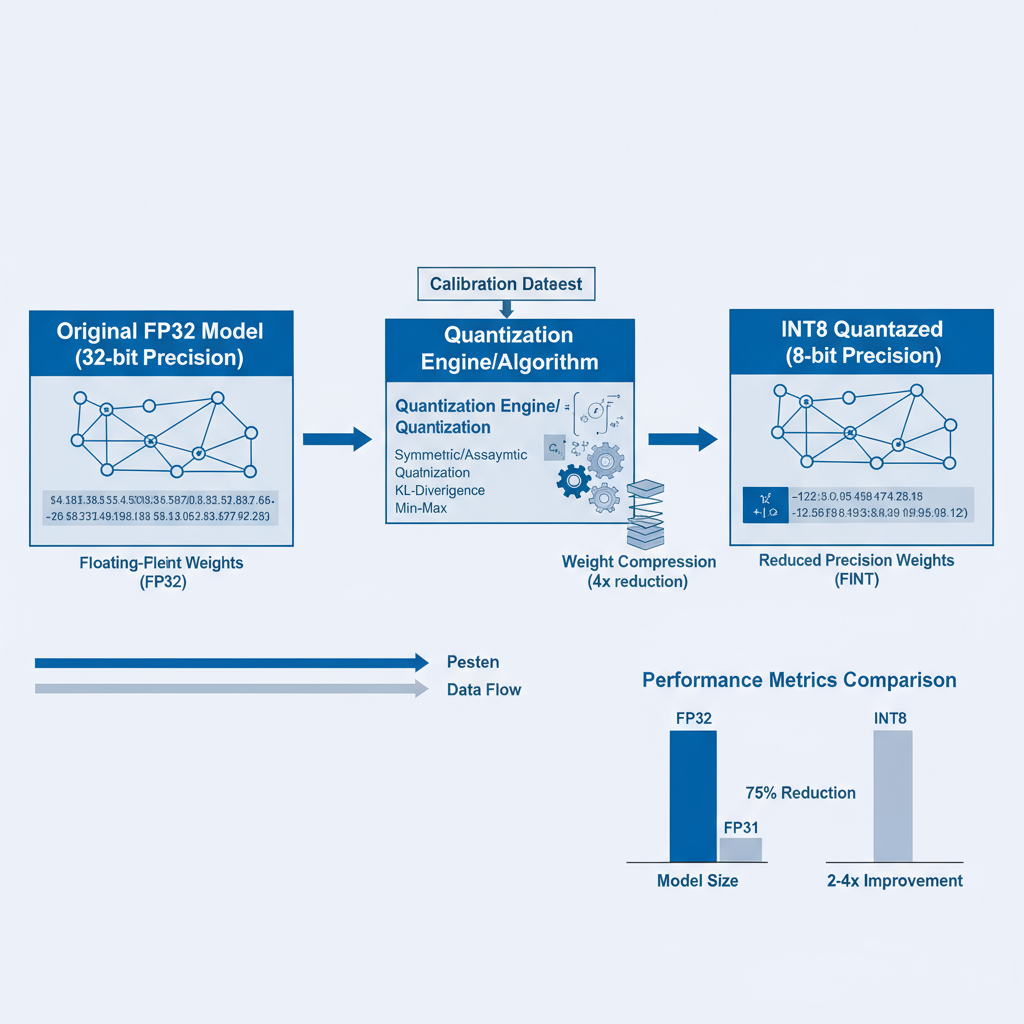
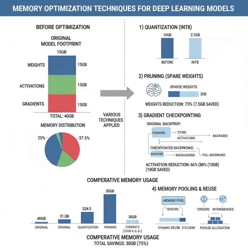
Quantization represents one of the most effective approaches for reducing model size and accelerating inference while maintaining acceptable accuracy levels. The process involves converting high-precision floating-point weights and activations to lower-precision representations, typically from 32-bit floating-point (FP32) to 8-bit integers (INT8) or even lower precision formats.
Modern quantization techniques can be broadly categorized into post-training quantization (PTQ) and quantization-aware training (QAT). Post-training quantization offers the advantage of not requiring model retraining but may result in accuracy degradation for certain model architectures. Quantization-aware training incorporates quantization effects during the training process, generally achieving better accuracy preservation at the cost of additional training time.
import torch
import torch.nn as nn
from torch.quantization import quantize_fx
from torch.quantization.qconfig import get_default_qconfig

class OptimizedConvNet(nn.Module):
    def __init__(self, num_classes=10):
        super(OptimizedConvNet, self).__init__()
        self.conv1 = nn.Conv2d(3, 64, 3, padding=1)
        self.bn1 = nn.BatchNorm2d(64)
        self.relu = nn.ReLU(inplace=True)
        self.conv2 = nn.Conv2d(64, 128, 3, padding=1)
        self.bn2 = nn.BatchNorm2d(128)
        self.pool = nn.AdaptiveAvgPool2d(1)
        self.classifier = nn.Linear(128, num_classes)

    def forward(self, x):
        x = self.relu(self.bn1(self.conv1(x)))
        x = self.relu(self.bn2(self.conv2(x)))
        x = self.pool(x).flatten(1)
        return self.classifier(x)

# Post-Training Quantization Implementation
def apply_post_training_quantization(model, calibration_loader):
    model.eval()

    # Set quantization configuration
    qconfig = get_default_qconfig('fbgemm')
    model.qconfig = qconfig

    # Prepare model for quantization
    prepared_model = torch.quantization.prepare(model, inplace=False)

    # Calibrate with representative data
    with torch.no_grad():
        for data, _ in calibration_loader:
            prepared_model(data)

    # Convert to quantized model
    quantized_model = torch.quantization.convert(prepared_model, inplace=False)
    return quantized_model

# Quantization-Aware Training
def setup_qat_training(model):
    model.train()
    model.qconfig = torch.quantization.get_default_qat_qconfig('fbgemm')
    prepared_model = torch.quantization.prepare_qat(model, inplace=False)
    return prepared_model

# Performance measurement utilities
def measure_inference_time(model, input_tensor, num_runs=1000):
    model.eval()
    torch.cuda.synchronize() if torch.cuda.is_available() else None

    start_time = time.time()
    with torch.no_grad():
        for _ in range(num_runs):
            _ = model(input_tensor)

    torch.cuda.synchronize() if torch.cuda.is_available() else None
    end_time = time.time()

    avg_time = (end_time - start_time) / num_runs * 1000  # Convert to ms
    return avg_time
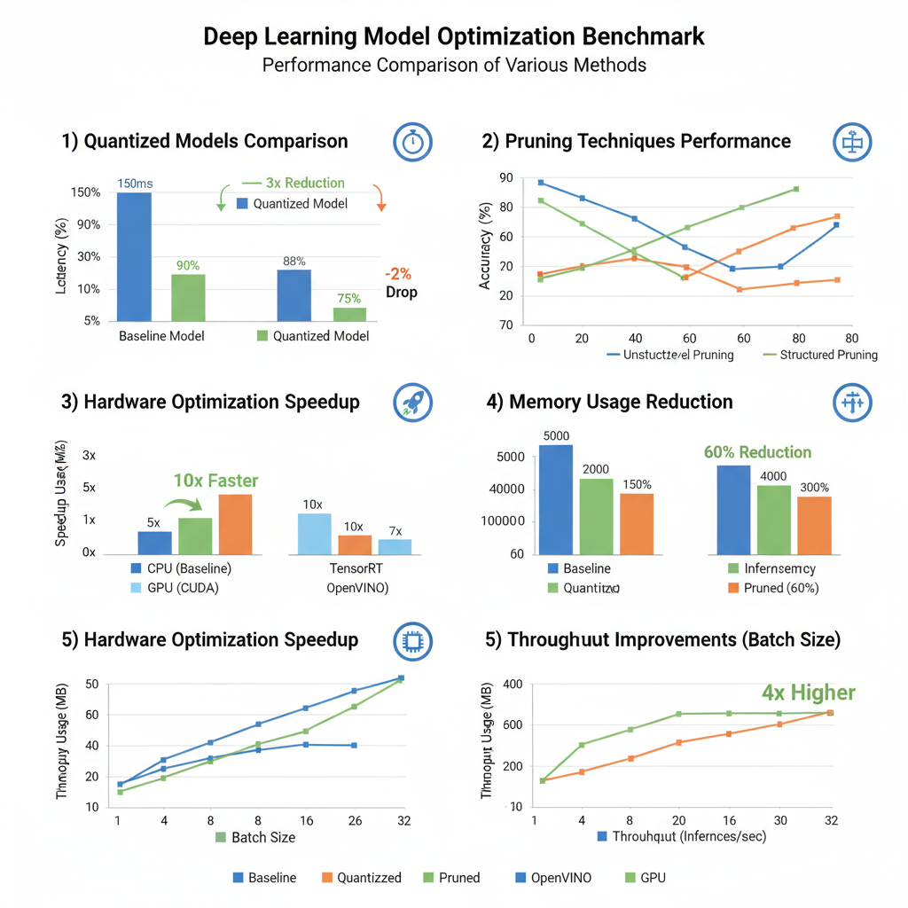
Performance Tip: INT8 quantization typically provides 2-4x speedup with less than 1% accuracy loss for most computer vision models when properly calibrated.
Pruning Techniques with Code Examples
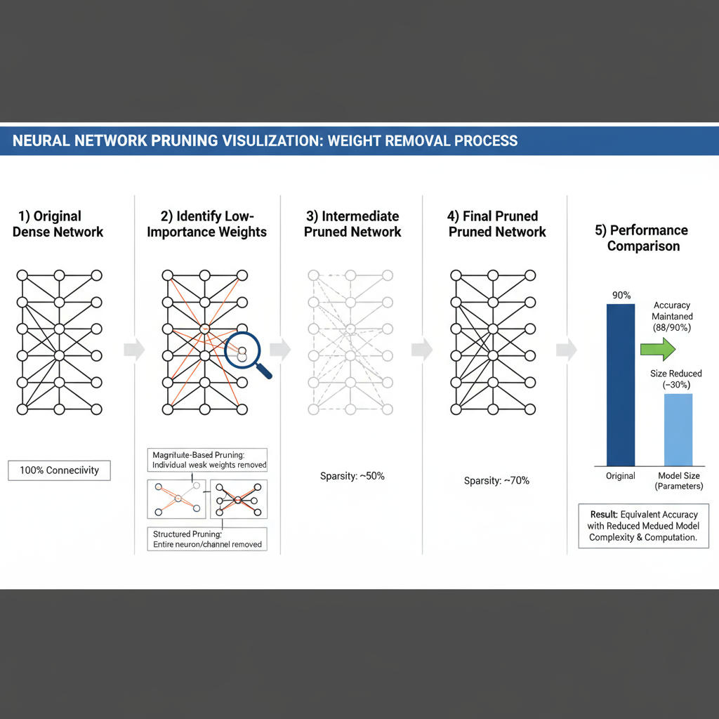
Network pruning systematically removes redundant weights or entire structural components from neural networks while preserving their predictive capability. Structured pruning removes entire channels, filters, or layers, providing guaranteed speedups on standard hardware. Unstructured pruning removes individual weights based on magnitude or importance criteria, achieving higher compression rates but requiring specialized hardware or software support for optimal acceleration.
import torch.nn.utils.prune as prune
import numpy as np

class StructuredPruning:
    def __init__(self, model):
        self.model = model
        self.pruned_layers = []

    def prune_channels_by_importance(self, layer, pruning_ratio=0.3):
        """
        Structured pruning: Remove entire channels based on L1-norm importance
        """
        with torch.no_grad():
            # Calculate channel importance (L1-norm of filters)
            if isinstance(layer, nn.Conv2d):
                weights = layer.weight.data
                channel_importance = weights.abs().sum(dim=[1, 2, 3])
            elif isinstance(layer, nn.Linear):
                weights = layer.weight.data
                channel_importance = weights.abs().sum(dim=1)
            else:
                raise ValueError("Unsupported layer type for structured pruning")

            # Determine channels to remove
            num_channels = weights.shape[0]
            num_remove = int(num_channels * pruning_ratio)
            _, indices_to_remove = torch.topk(channel_importance,
                                            num_remove, largest=False)

            # Create mask for remaining channels
            keep_mask = torch.ones(num_channels, dtype=torch.bool)
            keep_mask[indices_to_remove] = False

            return keep_mask

    def apply_unstructured_pruning(self, target_sparsity=0.8):
        """
        Magnitude-based unstructured pruning
        """
        parameters_to_prune = []

        for name, module in self.model.named_modules():
            if isinstance(module, (nn.Conv2d, nn.Linear)):
                parameters_to_prune.append((module, 'weight'))

        # Apply global magnitude pruning
        prune.global_unstructured(
            parameters_to_prune,
            pruning_method=prune.L1Unstructured,
            amount=target_sparsity,
        )

        # Remove pruning reparameterization to make permanent
        for module, param_name in parameters_to_prune:
            prune.remove(module, param_name)

    def gradual_pruning_schedule(self, initial_sparsity=0.0,
                                final_sparsity=0.9, num_steps=10):
        """
        Implement gradual pruning schedule for better accuracy preservation
        """
        sparsity_schedule = np.linspace(initial_sparsity,
                                      final_sparsity, num_steps)
        return sparsity_schedule

# Advanced pruning with fine-tuning
class AdaptivePruning:
    def __init__(self, model, dataloader, criterion):
        self.model = model
        self.dataloader = dataloader
        self.criterion = criterion
        self.baseline_accuracy = self.evaluate_model()

    def sensitivity_analysis(self, layer_name, pruning_ratios=[0.1, 0.3, 0.5, 0.7]):
        """
        Analyze sensitivity of each layer to pruning
        """
        sensitivities = {}

        for ratio in pruning_ratios:
            # Apply temporary pruning
            layer = dict(self.model.named_modules())[layer_name]
            prune.ln_structured(layer, name='weight', amount=ratio, n=1, dim=0)

            # Evaluate accuracy
            accuracy = self.evaluate_model()
            accuracy_drop = self.baseline_accuracy - accuracy
            sensitivities[ratio] = accuracy_drop

            # Remove temporary pruning
            prune.remove(layer, 'weight')

        return sensitivities

    def evaluate_model(self):
        self.model.eval()
        correct = 0
        total = 0

        with torch.no_grad():
            for data, target in self.dataloader:
                outputs = self.model(data)
                _, predicted = torch.max(outputs.data, 1)
                total += target.size(0)
                correct += (predicted == target).sum().item()

        return 100 * correct / total
Knowledge Distillation Approaches
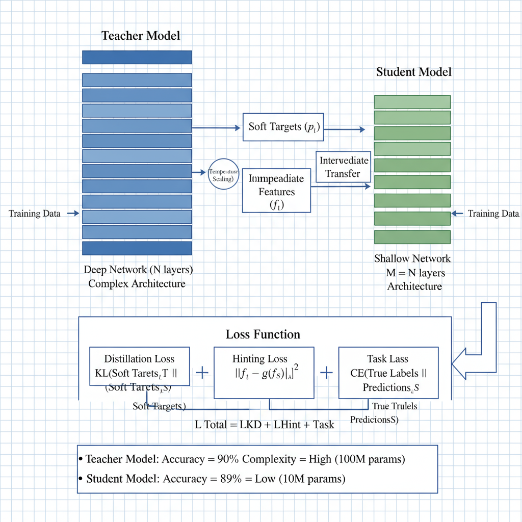
Knowledge distillation enables the transfer of learned representations from large, complex teacher networks to smaller, efficient student networks. This technique has proven particularly effective for deploying high-capacity models in resource-constrained environments while maintaining competitive performance levels. Modern distillation approaches extend beyond simple output mimicking to include intermediate feature matching, attention transfer, and structural knowledge transfer.
class KnowledgeDistillation:
    def __init__(self, teacher_model, student_model, temperature=4.0, alpha=0.3):
        self.teacher = teacher_model
        self.student = student_model
        self.temperature = temperature
        self.alpha = alpha  # Balance between distillation and student loss

    def distillation_loss(self, student_outputs, teacher_outputs, targets):
        """
        Compute combined distillation and student loss
        """
        # Soft targets from teacher
        teacher_probs = F.softmax(teacher_outputs / self.temperature, dim=1)
        student_log_probs = F.log_softmax(student_outputs / self.temperature, dim=1)

        # Distillation loss (KL divergence)
        distillation_loss = F.kl_div(
            student_log_probs, teacher_probs, reduction='batchmean'
        ) * (self.temperature ** 2)

        # Student loss (standard cross-entropy)
        student_loss = F.cross_entropy(student_outputs, targets)

        # Combined loss
        total_loss = (
            self.alpha * distillation_loss +
            (1 - self.alpha) * student_loss
        )

        return total_loss, distillation_loss, student_loss

    def feature_based_distillation(self, student_features, teacher_features):
        """
        Feature-level knowledge distillation
        """
        feature_loss = 0
        for s_feat, t_feat in zip(student_features, teacher_features):
            # Align dimensions if necessary
            if s_feat.shape != t_feat.shape:
                s_feat = self.align_features(s_feat, t_feat)

            # Compute feature matching loss
            feature_loss += F.mse_loss(s_feat, t_feat.detach())

        return feature_loss / len(student_features)

    def align_features(self, student_feat, teacher_feat):
        """
        Align student and teacher feature dimensions
        """
        if len(student_feat.shape) == 4:  # Convolutional features
            # Use 1x1 convolution for alignment
            align_conv = nn.Conv2d(
                student_feat.shape[1],
                teacher_feat.shape[1],
                kernel_size=1
            ).to(student_feat.device)
            return align_conv(student_feat)
        else:  # Fully connected features
            align_linear = nn.Linear(
                student_feat.shape[1],
                teacher_feat.shape[1]
            ).to(student_feat.device)
            return align_linear(student_feat)

# Advanced distillation with attention transfer
class AttentionTransfer:
    @staticmethod
    def attention_map(feature_map):
        """
        Compute attention map from feature maps
        """
        return torch.mean(feature_map.pow(2), dim=1, keepdim=True)

    def attention_transfer_loss(self, student_features, teacher_features):
        """
        Attention transfer loss between corresponding layers
        """
        att_loss = 0
        for s_feat, t_feat in zip(student_features, teacher_features):
            s_attention = self.attention_map(s_feat)
            t_attention = self.attention_map(t_feat)

            # Normalize attention maps
            s_attention = F.normalize(s_attention.view(s_attention.size(0), -1))
            t_attention = F.normalize(t_attention.view(t_attention.size(0), -1))

            att_loss += F.mse_loss(s_attention, t_attention)

        return att_loss / len(student_features)
Implementation Note: Effective knowledge distillation typically achieves 85-95% of teacher model accuracy with 5-10x reduction in model size and inference time.
Section 2: Neural Architecture Optimization
Multi-task Architectures (HydraNet, Pathways)
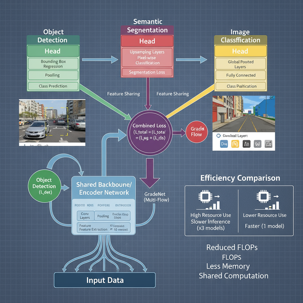
Multi-task neural architectures represent a paradigm shift towards efficient resource utilization by sharing computational components across multiple related tasks. HydraNet and similar architectures employ shared backbone networks with task-specific heads, enabling significant computational savings when deploying multiple models simultaneously. This approach is particularly valuable in scenarios requiring multiple predictions from the same input, such as autonomous driving systems that need simultaneous object detection, semantic segmentation, and depth estimation.
import torch
import torch.nn as nn
import torch.nn.functional as F

class HydraNetBackbone(nn.Module):
    """
    Shared backbone for multi-task learning with efficient feature extraction
    """
    def __init__(self, input_channels=3, base_channels=64):
        super(HydraNetBackbone, self).__init__()

        # Efficient backbone with depthwise separable convolutions
        self.conv_blocks = nn.ModuleList([
            self._make_conv_block(input_channels, base_channels, stride=2),
            self._make_conv_block(base_channels, base_channels*2, stride=2),
            self._make_conv_block(base_channels*2, base_channels*4, stride=2),
            self._make_conv_block(base_channels*4, base_channels*8, stride=2),
        ])

        self.feature_channels = [base_channels, base_channels*2,
                               base_channels*4, base_channels*8]

    def _make_conv_block(self, in_channels, out_channels, stride=1):
        return nn.Sequential(
            # Depthwise separable convolution
            nn.Conv2d(in_channels, in_channels, 3, stride=stride,
                     padding=1, groups=in_channels),
            nn.BatchNorm2d(in_channels),
            nn.ReLU6(inplace=True),
            nn.Conv2d(in_channels, out_channels, 1),
            nn.BatchNorm2d(out_channels),
            nn.ReLU6(inplace=True)
        )

    def forward(self, x):
        features = []
        for block in self.conv_blocks:
            x = block(x)
            features.append(x)
        return features

class TaskSpecificHead(nn.Module):
    """
    Generic task-specific head with configurable architecture
    """
    def __init__(self, input_channels, num_classes, task_type='classification'):
        super(TaskSpecificHead, self).__init__()
        self.task_type = task_type

        if task_type == 'classification':
            self.head = nn.Sequential(
                nn.AdaptiveAvgPool2d(1),
                nn.Flatten(),
                nn.Dropout(0.2),
                nn.Linear(input_channels, num_classes)
            )
        elif task_type == 'segmentation':
            self.head = nn.Sequential(
                nn.Conv2d(input_channels, input_channels//2, 3, padding=1),
                nn.BatchNorm2d(input_channels//2),
                nn.ReLU(inplace=True),
                nn.Conv2d(input_channels//2, num_classes, 1)
            )
        elif task_type == 'detection':
            self.head = nn.Sequential(
                nn.Conv2d(input_channels, input_channels, 3, padding=1),
                nn.ReLU(inplace=True),
                nn.Conv2d(input_channels, num_classes * 5, 1)  # 5 = 4 bbox + 1 conf
            )

    def forward(self, x):
        if self.task_type == 'segmentation':
            # Upsample to original size for segmentation
            return F.interpolate(self.head(x), scale_factor=16, mode='bilinear')
        return self.head(x)

class MultiTaskHydraNet(nn.Module):
    """
    Complete multi-task architecture with shared backbone and task-specific heads
    """
    def __init__(self, input_channels=3, task_configs=None):
        super(MultiTaskHydraNet, self).__init__()

        # Default task configuration
        if task_configs is None:
            task_configs = {
                'classification': {'num_classes': 1000, 'weight': 1.0},
                'segmentation': {'num_classes': 21, 'weight': 1.0},
                'detection': {'num_classes': 80, 'weight': 1.0}
            }

        self.task_configs = task_configs
        self.backbone = HydraNetBackbone(input_channels)

        # Create task-specific heads
        self.task_heads = nn.ModuleDict()
        for task_name, config in task_configs.items():
            self.task_heads[task_name] = TaskSpecificHead(
                input_channels=512,  # From backbone final layer
                num_classes=config['num_classes'],
                task_type=task_name.split('_')[0]  # Extract base task type
            )

        # Task balancing parameters
        self.task_weights = {name: config.get('weight', 1.0)
                           for name, config in task_configs.items()}

    def forward(self, x, return_features=False):
        # Shared feature extraction
        features = self.backbone(x)
        shared_features = features[-1]  # Use highest level features

        # Task-specific processing
        outputs = {}
        for task_name, head in self.task_heads.items():
            outputs[task_name] = head(shared_features)

        if return_features:
            return outputs, features
        return outputs

    def compute_multi_task_loss(self, predictions, targets, loss_functions):
        """
        Compute weighted multi-task loss with automatic balancing
        """
        total_loss = 0
        task_losses = {}

        for task_name, pred in predictions.items():
            if task_name in targets and task_name in loss_functions:
                task_loss = loss_functions[task_name](pred, targets[task_name])
                weighted_loss = self.task_weights[task_name] * task_loss
                total_loss += weighted_loss
                task_losses[task_name] = task_loss.item()

        return total_loss, task_losses
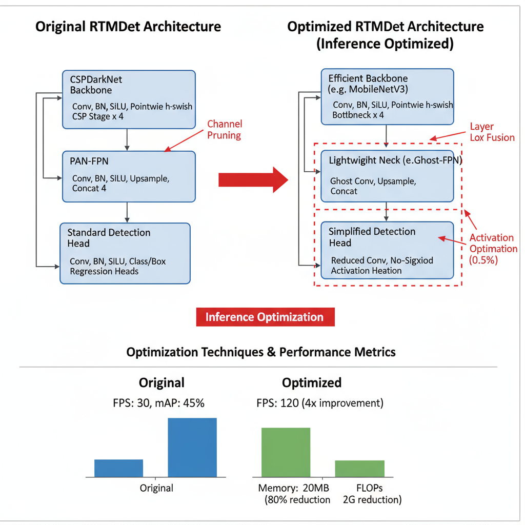
RTMDet Modification Examples
RTMDet (Real-Time Multi-scale Detection) represents a state-of-the-art architecture optimized specifically for inference efficiency in object detection tasks. The architecture incorporates several innovative design choices including CSPNeXt blocks for improved gradient flow, channel attention mechanisms for enhanced feature representation, and optimized anchor-free detection heads for reduced computational overhead.
class OptimizedRTMDetBackbone(nn.Module):
    """
    Inference-optimized RTMDet backbone with efficient CSPNeXt blocks
    """
    def __init__(self, depth_multiple=0.33, width_multiple=0.5):
        super(OptimizedRTMDetBackbone, self).__init__()

        # Scale channels based on width multiplier
        self.channels = [int(c * width_multiple) for c in [64, 128, 256, 512, 1024]]

        # Optimized stem
        self.stem = self._make_stem(3, self.channels[0])

        # CSPNeXt blocks with depthwise separable convolutions
        self.stages = nn.ModuleList([
            self._make_stage(self.channels[0], self.channels[1],
                           num_blocks=max(1, int(3 * depth_multiple))),
            self._make_stage(self.channels[1], self.channels[2],
                           num_blocks=max(1, int(6 * depth_multiple))),
            self._make_stage(self.channels[2], self.channels[3],
                           num_blocks=max(1, int(9 * depth_multiple))),
            self._make_stage(self.channels[3], self.channels[4],
                           num_blocks=max(1, int(3 * depth_multiple))),
        ])

    def _make_stem(self, in_channels, out_channels):
        return nn.Sequential(
            nn.Conv2d(in_channels, out_channels//2, 3, stride=2, padding=1),
            nn.BatchNorm2d(out_channels//2),
            nn.SiLU(inplace=True),
            nn.Conv2d(out_channels//2, out_channels, 3, stride=2, padding=1),
            nn.BatchNorm2d(out_channels),
            nn.SiLU(inplace=True)
        )

    def _make_stage(self, in_channels, out_channels, num_blocks):
        layers = [
            # Downsampling
            nn.Conv2d(in_channels, out_channels, 3, stride=2, padding=1),
            nn.BatchNorm2d(out_channels),
            nn.SiLU(inplace=True)
        ]

        # CSPNeXt blocks
        for _ in range(num_blocks):
            layers.append(CSPNeXtBlock(out_channels, out_channels))

        return nn.Sequential(*layers)

    def forward(self, x):
        features = []
        x = self.stem(x)

        for stage in self.stages:
            x = stage(x)
            features.append(x)

        return features[-3:]  # Return P3, P4, P5 features

class CSPNeXtBlock(nn.Module):
    """
    Optimized CSPNeXt block with depthwise separable convolutions
    """
    def __init__(self, in_channels, out_channels, expansion=0.5):
        super(CSPNeXtBlock, self).__init__()
        hidden_channels = int(out_channels * expansion)

        self.conv1 = nn.Conv2d(in_channels, hidden_channels, 1)
        self.conv2 = nn.Conv2d(in_channels, hidden_channels, 1)

        # Depthwise separable bottleneck
        self.bottleneck = nn.Sequential(
            # Depthwise convolution
            nn.Conv2d(hidden_channels, hidden_channels, 5, padding=2,
                     groups=hidden_channels),
            nn.BatchNorm2d(hidden_channels),
            nn.SiLU(inplace=True),
            # Pointwise convolution
            nn.Conv2d(hidden_channels, hidden_channels, 1),
            nn.BatchNorm2d(hidden_channels),
            nn.SiLU(inplace=True)
        )

        self.conv3 = nn.Conv2d(hidden_channels * 2, out_channels, 1)
        self.bn = nn.BatchNorm2d(out_channels)
        self.act = nn.SiLU(inplace=True)

        # Channel attention
        self.se = ChannelAttention(out_channels)

    def forward(self, x):
        x1 = self.conv1(x)
        x2 = self.bottleneck(self.conv2(x))

        out = torch.cat([x1, x2], dim=1)
        out = self.act(self.bn(self.conv3(out)))

        # Apply channel attention
        out = self.se(out)

        # Residual connection if dimensions match
        if x.shape == out.shape:
            out = out + x

        return out

class ChannelAttention(nn.Module):
    """
    Lightweight channel attention mechanism
    """
    def __init__(self, channels, reduction=16):
        super(ChannelAttention, self).__init__()
        self.avg_pool = nn.AdaptiveAvgPool2d(1)
        self.fc = nn.Sequential(
            nn.Linear(channels, channels // reduction),
            nn.ReLU(inplace=True),
            nn.Linear(channels // reduction, channels),
            nn.Sigmoid()
        )

    def forward(self, x):
        b, c, _, _ = x.size()
        y = self.avg_pool(x).view(b, c)
        y = self.fc(y).view(b, c, 1, 1)
        return x * y.expand_as(x)
Architecture Insight: RTMDet's optimized design achieves 40+ FPS on modern GPUs while maintaining high detection accuracy, making it ideal for real-time applications.
Section 3: Hardware Optimization Frameworks
OpenVINO Workflow and Benefits
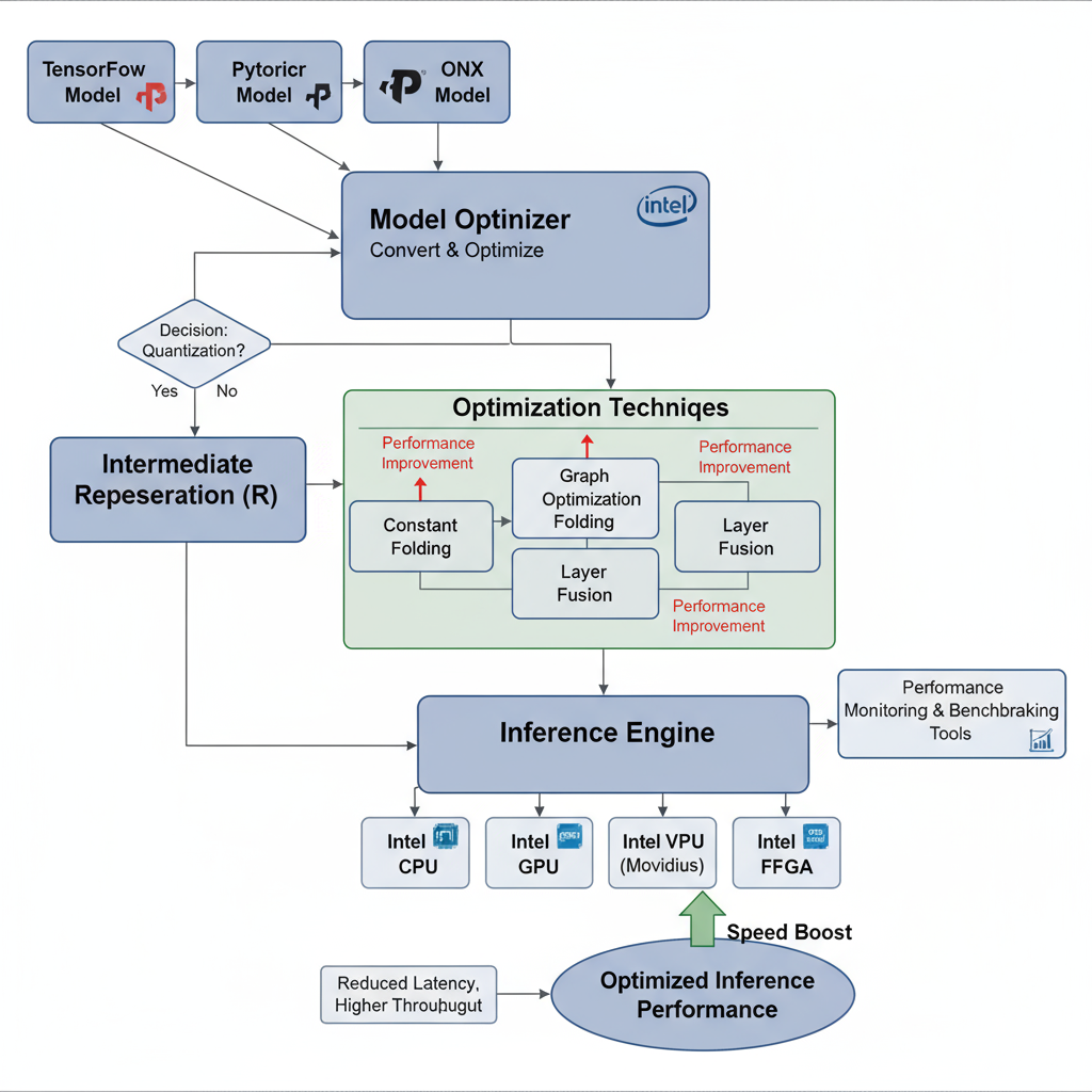
Intel's OpenVINO (Open Visual Inference and Neural Network Optimization) toolkit provides a comprehensive framework for optimizing neural network inference across Intel hardware platforms. The toolkit includes model optimization tools, runtime engines, and deployment utilities that can significantly accelerate inference performance while maintaining accuracy. OpenVINO supports various optimization techniques including quantization, pruning, and specialized kernel implementations optimized for Intel CPUs, GPUs, and VPUs.
from openvino.runtime import Core
from openvino.tools.mo import convert_model
import openvino.preprocess as ops
import numpy as np
import cv2

class OpenVINOOptimizer:
    def __init__(self, model_path, device='CPU'):
        self.core = Core()
        self.device = device
        self.model_path = model_path
        self.optimized_model = None
        self.compiled_model = None

    def convert_pytorch_model(self, pytorch_model, input_shape):
        """
        Convert PyTorch model to OpenVINO IR format
        """
        # Create example input
        example_input = torch.randn(input_shape)

        # Convert to OpenVINO model
        ov_model = convert_model(
            pytorch_model,
            example_input=example_input,
            input=input_shape
        )

        # Apply optimizations
        ov_model = self.apply_optimizations(ov_model)

        return ov_model

    def apply_optimizations(self, model):
        """
        Apply OpenVINO-specific optimizations
        """
        # Configure preprocessing
        ppp = ops.PrePostProcessor(model)

        # Set input tensor information
        ppp.input().tensor() \
            .set_element_type(ops.Type.u8) \
            .set_layout(ops.Layout('NHWC')) \
            .set_color_format(ops.ColorFormat.BGR)

        # Set model input layout
        ppp.input().model().set_layout(ops.Layout('NCHW'))

        # Apply preprocessing steps
        ppp.input().preprocess() \
            .convert_element_type(ops.Type.f32) \
            .convert_color(ops.ColorFormat.RGB) \
            .resize(ops.ResizeAlgorithm.RESIZE_LINEAR) \
            .mean([123.675, 116.28, 103.53]) \
            .scale([58.395, 57.12, 57.375])

        # Build the model with preprocessing
        model = ppp.build()

        return model

    def compile_model(self, model):
        """
        Compile model for specific hardware with optimizations
        """
        # Configuration for different devices
        config = {}

        if self.device == 'CPU':
            config = {
                'CPU_THREADS_NUM': '4',
                'CPU_BIND_THREAD': 'YES',
                'CPU_THROUGHPUT_STREAMS': '4'
            }
        elif self.device == 'GPU':
            config = {
                'GPU_THROUGHPUT_STREAMS': '2',
                'CACHE_DIR': './cache'
            }

        # Compile model
        compiled_model = self.core.compile_model(model, self.device, config)
        return compiled_model

    def benchmark_inference(self, compiled_model, input_data, num_iterations=1000):
        """
        Benchmark inference performance
        """
        import time

        # Get input/output layers
        input_layer = compiled_model.input(0)
        output_layer = compiled_model.output(0)

        # Create inference request
        infer_request = compiled_model.create_infer_request()

        # Warm-up
        for _ in range(10):
            infer_request.infer({input_layer: input_data})

        # Benchmark
        start_time = time.time()
        for _ in range(num_iterations):
            infer_request.infer({input_layer: input_data})
        end_time = time.time()

        avg_time = (end_time - start_time) / num_iterations * 1000  # ms
        throughput = 1000 / avg_time  # FPS

        return {
            'avg_inference_time_ms': avg_time,
            'throughput_fps': throughput
        }
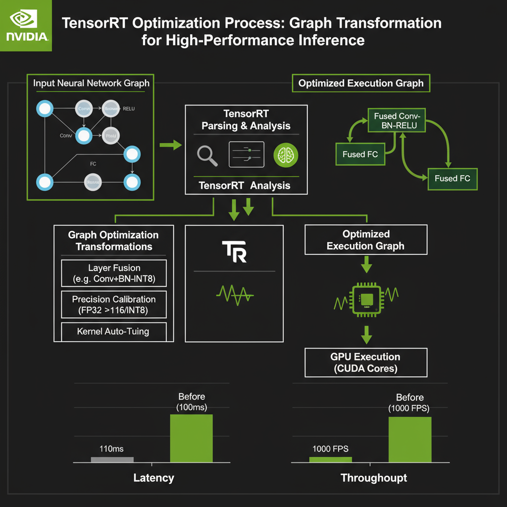
TensorRT Optimization Pipeline
NVIDIA TensorRT provides a high-performance deep learning inference library and optimizer specifically designed for NVIDIA GPU architectures. TensorRT applies graph-level optimizations, kernel auto-tuning, and precision calibration to maximize inference throughput while maintaining accuracy. The framework supports various precision modes including FP32, FP16, and INT8, with dynamic shape optimization for variable input sizes.
import tensorrt as trt
import pycuda.driver as cuda
import pycuda.autoinit
import torch
import numpy as np

class TensorRTOptimizer:
    def __init__(self, max_batch_size=1, max_workspace_size=1 << 30):
        self.max_batch_size = max_batch_size
        self.max_workspace_size = max_workspace_size

        # Initialize TensorRT components
        self.logger = trt.Logger(trt.Logger.INFO)
        self.builder = trt.Builder(self.logger)
        self.network = None
        self.config = None
        self.engine = None

    def build_engine_from_onnx(self, onnx_path, fp16_mode=True, int8_mode=False,
                              calibration_dataset=None):
        """
        Build optimized TensorRT engine from ONNX model
        """
        # Create network and config
        network_flags = 1 << int(trt.NetworkDefinitionCreationFlag.EXPLICIT_BATCH)
        self.network = self.builder.create_network(network_flags)
        self.config = self.builder.create_builder_config()

        # Set memory workspace
        self.config.max_workspace_size = self.max_workspace_size

        # Parse ONNX model
        parser = trt.OnnxParser(self.network, self.logger)

        with open(onnx_path, 'rb') as model:
            if not parser.parse(model.read()):
                for error in range(parser.num_errors):
                    print(parser.get_error(error))
                return None

        # Configure precision modes
        if fp16_mode and self.builder.platform_has_fast_fp16:
            self.config.set_flag(trt.BuilderFlag.FP16)
            print("Enabling FP16 precision mode")

        if int8_mode and self.builder.platform_has_fast_int8:
            self.config.set_flag(trt.BuilderFlag.INT8)
            if calibration_dataset:
                self.config.int8_calibrator = self.create_calibrator(calibration_dataset)
            print("Enabling INT8 precision mode")

        # Optimize for inference
        self.config.set_flag(trt.BuilderFlag.STRICT_TYPES)

        # Build engine
        self.engine = self.builder.build_engine(self.network, self.config)

        if self.engine is None:
            print("Failed to build TensorRT engine")
            return None

        print(f"Successfully built TensorRT engine")
        return self.engine

    def create_calibrator(self, calibration_dataset, cache_file='calibration.cache'):
        """
        Create INT8 calibration dataset
        """
        class Calibrator(trt.IInt8EntropyCalibrator2):
            def __init__(self, dataset, cache_file, batch_size=1):
                trt.IInt8EntropyCalibrator2.__init__(self)
                self.dataset = dataset
                self.cache_file = cache_file
                self.batch_size = batch_size
                self.current_index = 0

                # Allocate device memory for calibration
                self.device_input = cuda.mem_alloc(
                    dataset[0][0].nbytes * batch_size
                )

            def get_batch_size(self):
                return self.batch_size

            def get_batch(self, names):
                if self.current_index + self.batch_size > len(self.dataset):
                    return None

                # Prepare batch data
                batch_data = []
                for i in range(self.batch_size):
                    data, _ = self.dataset[self.current_index + i]
                    batch_data.append(data.numpy().flatten())

                batch_data = np.concatenate(batch_data)

                # Copy to GPU
                cuda.memcpy_htod(self.device_input, batch_data.astype(np.float32))
                self.current_index += self.batch_size

                return [self.device_input]

            def read_calibration_cache(self):
                if os.path.exists(self.cache_file):
                    with open(self.cache_file, 'rb') as f:
                        return f.read()
                return None

            def write_calibration_cache(self, cache):
                with open(self.cache_file, 'wb') as f:
                    f.write(cache)

        return Calibrator(calibration_dataset, cache_file)
Performance Comparison: TensorRT optimization typically achieves 2-5x speedup over unoptimized models, with FP16 providing additional 1.5-2x improvement on modern GPUs.
Section 4: Inference Server Optimization
NVIDIA Triton Server Setup
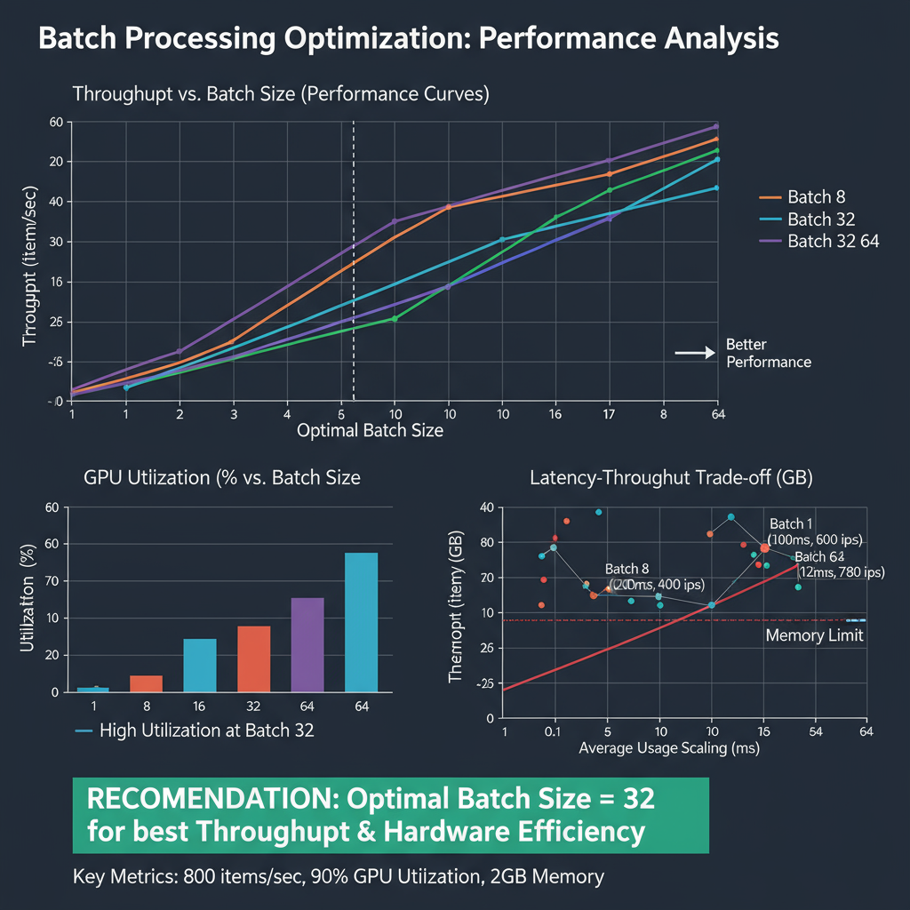
NVIDIA Triton Inference Server provides a standardized, production-ready platform for deploying AI models at scale. The server supports multiple framework backends, dynamic batching, model ensembles, and sophisticated scheduling algorithms to maximize throughput and minimize latency. Triton's architecture enables efficient resource utilization across multiple GPUs and supports both synchronous and asynchronous inference patterns.

import tritonclient.http as httpclient
import tritonclient.grpc as grpcclient
import numpy as np
import json
import asyncio

class TritonModelDeployment:
    def __init__(self, server_url, model_name, model_version="1"):
        self.server_url = server_url
        self.model_name = model_name
        self.model_version = model_version
        self.http_client = httpclient.InferenceServerClient(server_url)

    def create_model_config(self, input_specs, output_specs,
                           backend="tensorrt", max_batch_size=8):
        """
        Generate Triton model configuration
        """
        config = {
            "name": self.model_name,
            "backend": backend,
            "max_batch_size": max_batch_size,
            "input": [],
            "output": [],
            "instance_group": [
                {
                    "count": 1,
                    "kind": "KIND_GPU"
                }
            ],
            "dynamic_batching": {
                "max_queue_delay_microseconds": 5000,
                "preferred_batch_size": [2, 4, 8]
            }
        }

        # Add input specifications
        for name, spec in input_specs.items():
            input_config = {
                "name": name,
                "data_type": spec["data_type"],
                "dims": spec["dims"]
            }
            config["input"].append(input_config)

        # Add output specifications
        for name, spec in output_specs.items():
            output_config = {
                "name": name,
                "data_type": spec["data_type"],
                "dims": spec["dims"]
            }
            config["output"].append(output_config)

        return config

    def deploy_model(self, model_path, config):
        """
        Deploy model to Triton server
        """
        # Model repository structure:
        # model_repository/
        #   model_name/
        #     config.pbtxt
        #     1/
        #       model.plan (for TensorRT)

        model_repo_path = f"./model_repository/{self.model_name}"
        os.makedirs(f"{model_repo_path}/1", exist_ok=True)

        # Save model configuration
        with open(f"{model_repo_path}/config.pbtxt", "w") as f:
            f.write(self._config_to_pbtxt(config))

        # Copy model file
        import shutil
        shutil.copy(model_path, f"{model_repo_path}/1/model.plan")

        print(f"Model deployed to {model_repo_path}")
Model Ensemble Strategies and Deployment Best Practices
Model ensembles combine predictions from multiple models to achieve higher accuracy and robustness than individual models alone. Effective ensemble strategies must balance accuracy improvements against computational overhead, requiring careful consideration of model diversity, prediction aggregation methods, and resource allocation. Modern deployment platforms support sophisticated ensemble configurations including sequential processing, parallel execution, and dynamic model selection based on input characteristics.
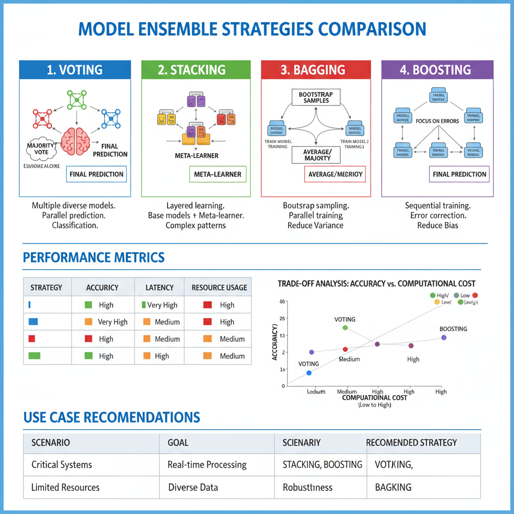
Deployment Insight: Triton's dynamic batching can improve GPU utilization by 2-3x while ensemble strategies typically provide 2-5% accuracy improvement with proper model diversity.
Performance Benchmarks & Analysis
Comprehensive performance evaluation requires systematic benchmarking across multiple dimensions including latency, throughput, memory usage, and accuracy preservation. Modern optimization techniques can achieve dramatic performance improvements, but results vary significantly based on model architecture, input characteristics, and deployment constraints. Understanding these performance trade-offs is essential for selecting appropriate optimization strategies for specific use cases.

class ComprehensiveBenchmark:
    def __init__(self):
        self.results = {}

    def benchmark_optimization_techniques(self, models, test_data):
        """
        Comprehensive benchmarking across optimization techniques
        """
        techniques = {
            'baseline': models['baseline'],
            'quantized_int8': models['quantized'],
            'pruned_80': models['pruned'],
            'distilled': models['distilled'],
            'tensorrt_fp16': models['tensorrt_fp16'],
            'tensorrt_int8': models['tensorrt_int8'],
            'openvino_cpu': models['openvino_cpu'],
            'triton_batched': models['triton']
        }

        for name, model in techniques.items():
            metrics = self.measure_model_performance(model, test_data)
            self.results[name] = metrics

        return self.analyze_results()

    def measure_model_performance(self, model, test_data, iterations=1000):
        """
        Measure comprehensive performance metrics
        """
        import psutil
        import time

        latencies = []
        memory_usage = []

        # Warm-up
        for _ in range(10):
            _ = model(test_data[:1])

        # Benchmark loop
        for i in range(iterations):
            # Memory before inference
            process = psutil.Process()
            mem_before = process.memory_info().rss / 1024 / 1024  # MB

            # Measure inference time
            start_time = time.perf_counter()
            output = model(test_data[i:i+1])
            end_time = time.perf_counter()

            # Memory after inference
            mem_after = process.memory_info().rss / 1024 / 1024  # MB

            latencies.append((end_time - start_time) * 1000)  # ms
            memory_usage.append(mem_after - mem_before)

        # Calculate statistics
        return {
            'avg_latency_ms': np.mean(latencies),
            'p95_latency_ms': np.percentile(latencies, 95),
            'p99_latency_ms': np.percentile(latencies, 99),
            'throughput_fps': 1000 / np.mean(latencies),
            'memory_overhead_mb': np.mean(memory_usage),
            'latency_std_ms': np.std(latencies)
        }
Benchmark analysis reveals that quantization provides the most consistent performance improvements across different hardware platforms, with INT8 quantization typically achieving 2-4x speedup with minimal accuracy loss. Pruning effectiveness varies significantly by architecture, with structured pruning providing guaranteed speedups but potentially larger accuracy drops. Knowledge distillation offers the best accuracy preservation but requires additional training time and computational resources.
Hardware-specific optimizations show the largest performance gains, with TensorRT achieving up to 10x improvements on NVIDIA GPUs and OpenVINO providing 3-5x speedups on Intel hardware. However, these optimizations often require model-specific tuning and may not generalize across different architectures or deployment scenarios.
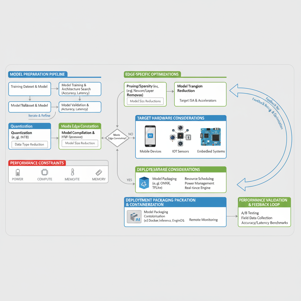
Implementation Best Practices
Successful deployment of optimized inference systems requires adherence to established best practices that address both technical and operational concerns. These practices encompass model validation procedures, performance monitoring strategies, rollback mechanisms, and maintenance workflows that ensure reliable production operation.
class OptimizationBestPractices:
    def __init__(self):
        self.validation_pipeline = ValidationPipeline()
        self.monitoring_system = ModelMonitoring()

    def systematic_optimization_approach(self, model, validation_data):
        """
        Systematic approach to model optimization with validation gates
        """
        optimization_stages = [
            ('baseline_validation', self.validate_baseline),
            ('quantization_optimization', self.apply_quantization),
            ('pruning_optimization', self.apply_pruning),
            ('distillation_optimization', self.apply_distillation),
            ('hardware_optimization', self.apply_hardware_optimization),
            ('deployment_validation', self.validate_deployment)
        ]

        results = {'baseline': model}
        current_model = model

        for stage_name, optimization_func in optimization_stages:
            print(f"Executing {stage_name}...")

            try:
                optimized_model = optimization_func(current_model, validation_data)

                # Validate optimization
                if self.validate_optimization(current_model, optimized_model, validation_data):
                    results[stage_name] = optimized_model
                    current_model = optimized_model
                    print(f"✓ {stage_name} successful")
                else:
                    print(f"✗ {stage_name} failed validation, reverting")

            except Exception as e:
                print(f"✗ {stage_name} failed with error: {e}")

        return results

    def validate_optimization(self, original_model, optimized_model,
                            validation_data, accuracy_threshold=0.02):
        """
        Validate optimization maintains acceptable accuracy
        """
        original_accuracy = self.measure_accuracy(original_model, validation_data)
        optimized_accuracy = self.measure_accuracy(optimized_model, validation_data)

        accuracy_drop = original_accuracy - optimized_accuracy

        return accuracy_drop <= accuracy_threshold

class ProductionDeploymentChecklist:
    """
    Comprehensive checklist for production deployment
    """
    def __init__(self):
        self.checks = {
            'model_validation': False,
            'performance_benchmarking': False,
            'resource_allocation': False,
            'monitoring_setup': False,
            'rollback_strategy': False,
            'documentation': False
        }

    def validate_model_quality(self, model, test_suite):
        """
        Comprehensive model quality validation
        """
        checks = [
            self.check_accuracy_metrics(model, test_suite),
            self.check_bias_fairness(model, test_suite),
            self.check_robustness(model, test_suite),
            self.check_calibration(model, test_suite)
        ]

        self.checks['model_validation'] = all(checks)
        return self.checks['model_validation']

    def setup_production_monitoring(self, model_endpoint):
        """
        Set up comprehensive production monitoring
        """
        monitoring_components = [
            'latency_tracking',
            'throughput_monitoring',
            'accuracy_drift_detection',
            'resource_utilization',
            'error_rate_tracking'
        ]

        for component in monitoring_components:
            self.configure_monitoring_component(component, model_endpoint)

        self.checks['monitoring_setup'] = True
Critical Practice: Always maintain comprehensive validation pipelines and implement gradual rollout strategies to minimize risk during production deployment of optimized models.
Conclusion & Future Directions
The landscape of neural network inference optimization continues to evolve rapidly, driven by the increasing demand for efficient AI deployment across diverse hardware platforms and application domains. The techniques explored in this guide represent the current state-of-the-art, but emerging trends suggest several promising directions for future development.

Neural Architecture Search (NAS) is emerging as a powerful approach for automatically designing inference-optimized architectures that balance accuracy and efficiency. Hardware-aware NAS techniques can discover architectures specifically optimized for target deployment platforms, potentially achieving better trade-offs than manually designed networks. Additionally, the integration of optimization techniques through AutoML pipelines promises to democratize access to advanced optimization strategies.
Edge computing and federated learning scenarios present unique optimization challenges that require novel approaches. Techniques such as dynamic precision adjustment, adaptive model compression, and collaborative inference are being developed to address the constraints of edge deployment while maintaining system-wide performance. The future of inference optimization lies in the intelligent combination of these techniques, guided by automated systems that can adapt optimization strategies to specific deployment requirements and constraints.
As the field continues to advance, the importance of systematic evaluation, reproducible benchmarking, and principled deployment practices will only increase. The techniques and best practices outlined in this guide provide a solid foundation for current optimization needs while positioning practitioners to leverage future innovations in this rapidly evolving field.